


FPW Group · Education Hub
Borrowing Capacity in Australia: How Much Can You Borrow for an Investment Property?
The most consistent surprise for Australian property investors in 2026 is not what the market has done. It is what the bank will not approve.
Incomes have grown. Property values have recovered across most capital city markets. Interest rates have moved off their 2023 peak. Yet the approved loan amounts coming back from lenders are materially lower than they were four years ago, often by $300,000 to $500,000 on identical income profiles.
What moved was the architecture of how banks measure risk. Understanding borrowing capacity as a constraint separate from asset pricing, and understanding the debt-to-income ratio framework that now sits on top of it, is where serious property investment strategy in 2026 has to start.
Australia's housing affordability problem has increasingly become a financing problem, not simply a pricing problem. The median Australian household has not become less creditworthy. It has become subject to assessment assumptions that would have made a 2019 mortgage significantly harder to approve.

In a Nutshell - If you only remember a few things:
Banks assess your loan at approximately 9.5 per cent, not your actual interest rate. That gap is structural, not temporary.
APRA's DTI cap now limits high-debt borrowing at a system level, not just at individual lender discretion.
Rental income is typically discounted to 70 to 80 per cent by lenders. Your portfolio's actual returns count for less than you think.
Existing debts and credit card limits reduce borrowing power whether you use them or not.
Equity helps with deposits. Income determines borrowing power. The two constraints operate independently.
Most investors in 2026 are constrained by serviceability, DTI ratios, and lender policy, not just property prices.
Table of contents
What Is the Debt-to-Income Ratio: APRA's February 2026 framework and what changed
How Equity Affects Borrowing Capacity: Why paper wealth does not solve the income problem
Borrowing Capacity vs Serviceability: Why the distinction matters practically
Can You Still Build a Property Portfolio in Australia in 2026?
Final Thoughts on Borrowing Capacity and Property Investment
What Is Borrowing Capacity?
Borrowing capacity is the maximum loan amount a lender will approve based on their assessment of your ability to service that debt under adverse conditions.
The bank is not assessing your ability to meet repayments at the rate they are offering you. It is assessing your ability to meet repayments at a rate considerably higher than that, while applying benchmarks for your living expenses that may exceed what you actually spend.
That double compression is why the number that comes back from a credit assessment is reliably lower than what borrowers calculate themselves.
What changed since the low-rate era is not the concept. Banks have always stress-tested borrowers. What changed is the magnitude of the stress, and the addition of a second framework that operates as a structural ceiling entirely separate from the serviceability calculation.
A borrower today does not face one constraint. They face two, running simultaneously.
What This Means in Practice
Borrowing capacity is the output of a model, one where lenders apply conservative assumptions at every input.
The gap between what you think you can borrow and what the bank approves is a feature of the system, not a negotiating error.
Understanding why the number is what it is, starting with the borrowing capacity formula, is the first step to changing it.
How Banks Calculate Borrowing Capacity
Most borrowers understand the basic inputs: income, expenses, existing debt. What they underestimate is how conservatively each input is treated, and how that conservative treatment compounds into a much lower approved figure.
Income: What Counts and How Much of It
PAYG income is generally accepted at full value. Everything beyond that involves discounting. Self-employed income is averaged over two years, often at a lower figure than the most recent year, then commonly shaded further.
For investors, rental income is the critical variable. Most lenders accept only 70 to 80 per cent of gross rental receipts in the serviceability model. The implied logic is that vacancy, maintenance, and management costs erode effective returns below gross figures.
For an investor generating $60,000 per year in gross rent across two properties, the lender's assessment might count $42,000 to $48,000 of that. That gap accumulates across a portfolio and becomes one of the primary reasons investors hit their capacity ceiling earlier than their apparent income would suggest.
The Household Expenditure Measure (HEM): The Floor Many Borrowers Do Not See
Banks benchmark declared living expenses against the Household Expenditure Measure, a statistical estimate of household spending that scales with income and family composition. The lender uses whichever figure is higher.
For higher-income households, the HEM benchmark frequently exceeds actual spending by a meaningful margin. There is no way to override the benchmark below the declared figure.
The gap directly reduces the surplus income available to service new debt, invisibly and without negotiation.
The Serviceability Buffer: The Most Consequential Policy Setting in Australian Lending
Every home loan in Australia is assessed at a rate three percentage points above the actual loan rate. APRA confirmed this setting would remain unchanged in July 2025.
At a current variable rate of around 6.5 per cent, that places the assessment rate at approximately 9.5 per cent. On a $700,000 loan over 30 years, the assessed monthly repayment at 9.5 per cent is approximately $5,880, compared to $4,420 at the actual market rate.
The lender requires the borrower to demonstrate capacity to service a loan that costs $1,460 more per month than the one being approved.
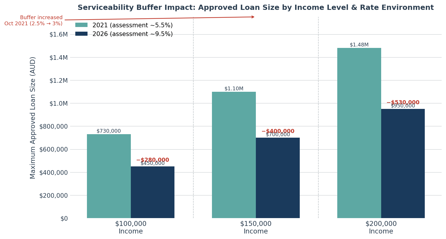
The same income profile that supported a $1.1 million loan in 2021 now supports roughly $700,000, a reduction of around $400,000 with no change in the borrower's financial position. The entire compression is a function of the three-point assessment buffer applied to a higher base rate, not a shift in creditworthiness.
Investors waiting for rate cuts to restore borrowing capacity should note that a 50 basis point cut reduces the assessment rate by exactly 50 basis points — meaningful, but not a recovery from the scale of compression shown here.
Source: Modelled scenario. APRA serviceability buffer settings confirmed July 2025.
The buffer was designed to prevent borrowers from stretching too far during low-rate periods. After 2022 and 2023, that design proved its purpose. The question is what it costs investors to live inside it permanently.
What This Means in Practice
The serviceability buffer is not a temporary caution. It is a permanent structural feature of Australian lending that APRA has shown no intention of removing.
Investors waiting for conditions to ease before their next acquisition may be waiting for a change that is not coming.
The smarter move is to plan around the buffer by structuring income, debt, and lender selection to maximise the surplus the bank's model actually sees.
What Is the Debt-to-Income Ratio?
Australia's lending environment shifted structurally in February 2026 when APRA activated a formal debt-to-income ratio lending limit. It had existed only as a threat for years. That changed.
The ratio is total outstanding debt divided by gross annual income. A household earning $200,000 with $1.4 million in total debt carries a DTI of seven times.
Under the framework from 1 February 2026, lenders can issue no more than 20 per cent of new mortgage lending to borrowers at or above a DTI of six times. That 20 per cent quota applies separately to owner-occupier and investor portfolios.
Why APRA Moved When It Did
Investor lending had been the primary driver of high-DTI growth. In the September quarter of 2025, investor loans at or above the six-times threshold reached around 10 per cent of new investor lending, up from 8 per cent a year earlier.
Total investor lending hit a record $72 billion in new commitments during that quarter alone. APRA moved before the trend could accelerate further.
That is consistent with how it has operated across every previous tightening cycle. It acts early, with tools it has prepared in advance.
What the DTI Cap Actually Does
The cap does not prohibit high-DTI lending. It introduces a system-level quota that individual lenders must manage across their quarterly books. The practical implication is less visible than a direct denial, and more consequential for it. Understanding how it affects high-income investors specifically requires recognising that high income does not exempt a borrower from the six-times threshold.
A household earning $350,000 with $2.1 million in total debt carries exactly the same DTI as one earning $100,000 with $600,000 in debt. The ratio is scale-invariant. That is a structural feature, not an oversight.
New construction loans are exempt from the cap. That carve-out aligns the DTI framework with the 2026 federal budget's housing supply objectives and creates a structural advantage for investors oriented toward new dwellings.
Calculating DTI and Reading What It Reveals
Knowing how to calculate your debt-to-income ratio is the starting point for understanding which constraint is actually binding on your next application. Both serviceability and DTI apply simultaneously.
The calculation includes credit card limits at their full limit value, not balance. An investor with $50,000 in credit limits across unused cards has $50,000 in assessed debt that contributes nothing to income.
That inclusion is the most commonly missed variable in investor DTI self-assessments. It is also one of the easiest to fix.
Run both calculations before every acquisition. Investors focused on only one tend to be blindsided by the other.
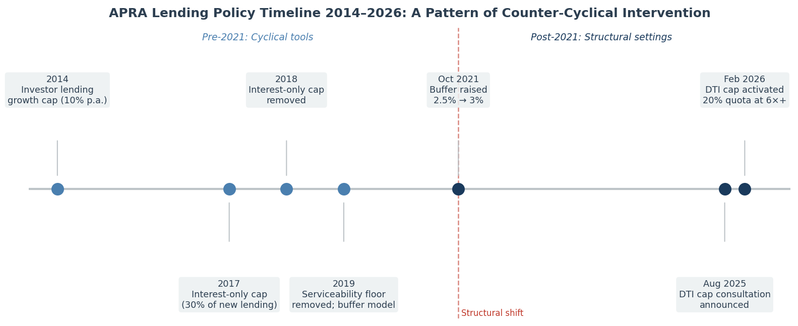
The February 2026 DTI cap is not a one-off policy response; it is the seventh significant macro-prudential intervention in twelve years.
APRA has consistently acted before lending growth reaches systemic risk levels, then held its settings longer than the market expects. Investors who treated each previous tightening as temporary and waited for settings to relax often found conditions had shifted before they re-entered the market.
Source: APRA policy releases 2014 to 2026.
What This Means in Practice
The DTI cap and serviceability buffer address different dimensions of risk.
Serviceability tests cash flow adequacy under stress. DTI tests structural leverage relative to income.
Both can bind on the same application. Investors who track only one constraint tend to encounter the other at the worst possible moment.
How Much Can You Borrow for an Investment Property?
The most honest framing of this question is not a number. It is a gap. The gap between what borrowers expect based on their income and assets, and what the current lending architecture will actually approve.
The Rate Cycle Compression
A single borrower earning $150,000 with no existing debt, applying in 2021 at a stress-test rate of approximately 5.5 per cent, might have qualified for $1.1 million to $1.2 million.
The same borrower applying today, on the same income, is assessed at 9.5 per cent and typically qualifies for $700,000 to $800,000. Nothing about their financial position changed. The assessment framework did.
That $400,000 reduction is not primarily a consequence of interest rates being higher. It is the consequence of a three-point buffer being applied to a higher base rate.
When rates were 2.5 per cent, the buffer pushed the assessment to 5.5 per cent. Now that rates sit at around 6.5 per cent, the buffer pushes the assessment to 9.5 per cent. The buffer percentage is identical. The dollar impact is not.
Many investors now face a paradox where property values have recovered or exceeded 2022 peaks, but borrowing capacity has not recovered in proportion. You can be wealthier on paper and less able to borrow.
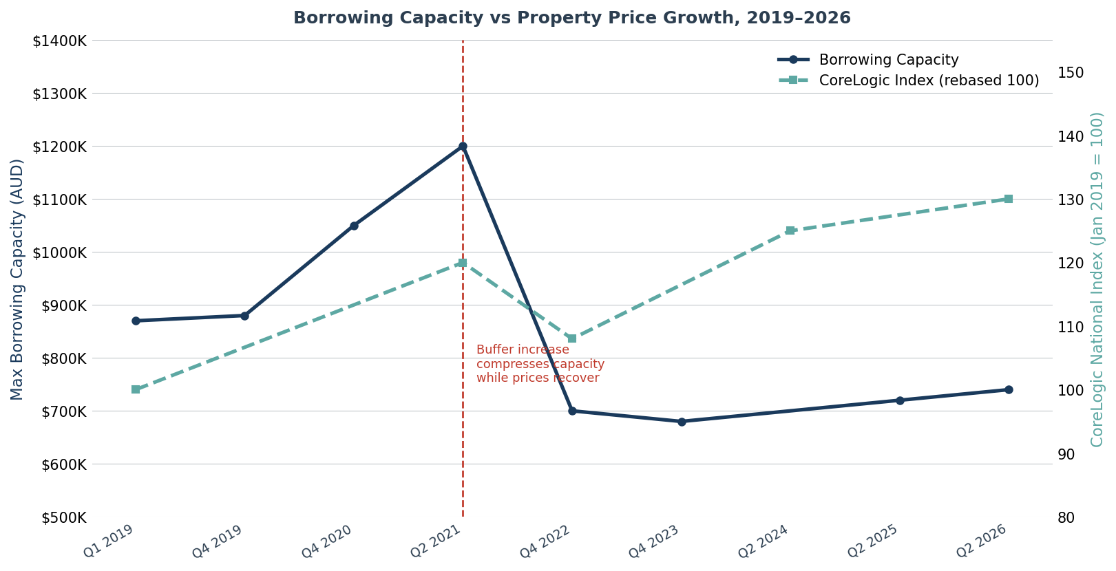
Property values nationally recovered from their 2022 lows and moved above previous peaks by mid-2024, but borrowing capacity did not follow the same trajectory.
The divergence from late 2021 onward reflects the buffer increase in October 2021, prices adjusted slowly while borrowing capacity compressed sharply. An investor re-entering the market in 2026 faces a wider gap between what they can buy and what the bank will approve than at any point in the prior decade.
Source: CoreLogic Home Value Index, national series. Modelled borrowing capacity under APRA assessment settings. Median Australian household income assumed at $130,000.
Where the Compression Concentrates for Portfolio Investors
Single-property analysis understates the problem. An investor with two existing loans has a compounding structure where each additional property adds debt at full assessed value but contributes rental income at only 70 to 80 per cent.
An investor on $250,000 household income with three properties carrying $1.8 million in combined debt runs an implied annual repayment obligation of approximately $170,000 through the bank's stress-test model, before living expense benchmarks are applied. The surplus available to service a fourth loan is already narrow. Add the DTI calculation and they are sitting at 7.2 times. That distinction matters when choosing the right investment property in 2026.
Not a bad credit risk. A structurally constrained one.
What This Means in Practice
Borrowing capacity is not just a function of income. It is a function of how the lender treats that income across a specific portfolio structure at a specific point in time.
Two borrowers with identical gross earnings can receive materially different credit assessments depending on whether their income is PAYG or self-employed, how many investment properties they hold, and which lender they are applying through.
The implication is that lender selection and debt restructuring are as important as income growth in expanding the ceiling.
How to Increase Borrowing Capacity
The practical work of expanding borrowing capacity happens mostly before a loan application. It sits in the structure of existing debt, the composition of the lender's credit model, and the specific adjustments that shift the assessed surplus income upward. For a detailed breakdown, see what determines your borrowing capacity.
Cancel the Credit Exposure That Is Not Earning Anything
Credit card limits are assessed as debt in full, regardless of utilisation. An investor with $80,000 in credit limits across cards they rarely use has $80,000 in assessed debt generating no return and requiring no income offset.
Cancelling or consolidating those limits before an application reduces total assessed debt and improves both the serviceability calculation and the DTI ratio simultaneously.
This is the clearest example in property finance of a change that costs nothing and produces an immediate modelling benefit.
Match the Lender's Credit Model to Your Income Structure
Lender policy on income assessment varies more than most borrowers realise. Some lenders accept 80 per cent of self-employed income averaged over two years. Others accept 100 per cent where recent business financials show consistent performance.
Some shade rental income to 70 per cent across all investor profiles. Others apply 75 or 80 per cent for investors with fewer than four properties, tightening the rate for larger portfolios.
The difference across lenders on a $50,000 gross rental income, assessed at either $35,000 or $40,000, is not trivial when compounded through a serviceability model.
Restructure Existing Debt Ahead of the Next Acquisition
An interest-only term on an existing investment loan reduces the assessed monthly repayment obligation in the bank's model, improving the residual surplus available to service new debt. A refinance of investment loans executed three to six months before a new purchase is meaningfully more effective than restructuring after a contract is signed.
Most investors approach each acquisition as a standalone event. It is better understood as maintenance on a portfolio finance structure that depreciates in efficiency as debt accumulates.
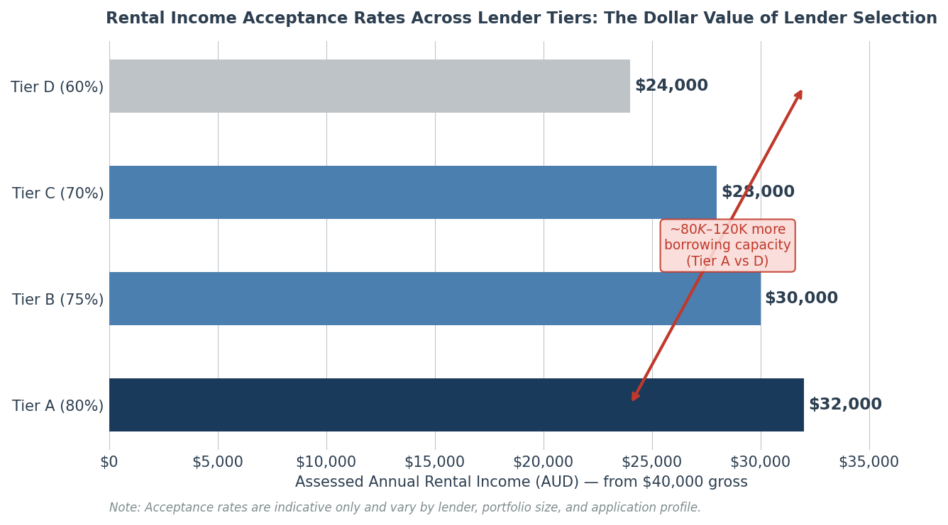
On the same $40,000 gross rental income, the difference between a Tier A lender (80 per cent acceptance) and a Tier D lender (60 per cent) is $8,000 in assessed annual income.
Run through a serviceability model at the 9.5 per cent assessment rate, that variance translates into approximately $80,000 to $120,000 in additional approved loan capacity. This is for the same borrower, same income, same property.
Lender selection is not an administrative detail. It is a structural lever that moves the ceiling.
Source: Indicative lender policy ranges, 2026. Based on modelled serviceability assessment at 9.5% assessment rate.
What This Means in Practice
Lender selection is a strategic decision, not an administrative one.
The lender policy matrices that govern income shading, rental income acceptance, and DTI thresholds are not publicly available.
This is where an investor-focused mortgage broker earns their engagement, not in sourcing a competitive rate, but in matching the right lender model to the borrower's specific income structure.
Does Existing Debt Reduce Borrowing Power?
Yes. Directly, mechanically, and in a way that compounds with each additional acquisition.
Bank serviceability models do not primarily assess how successful a portfolio appears on paper. They assess whether total debt obligations remain serviceable under stressed lending assumptions.
Every outstanding loan is assessed using the lender's assessment rate, not the actual repayment rate. The model then tests whether sufficient income surplus remains after all liabilities, living expenses, and repayment obligations are accounted for.
A property with strong rental yield and low LVR may improve servicing outcomes through additional rental income, but the associated debt is still included in full within the assessment model.
As portfolio debt rises, borrowing capacity generally declines unless income growth or cash flow improvements offset the additional repayment burden.
The borrowing capacity formula means that operational success in property investment does not translate linearly into increased credit access. Investors sometimes discover this when a strong-performing portfolio fails to support a fourth acquisition despite producing returns that would appear to justify it. That is one of the more disorienting moments in portfolio building.
Two Constraints Running Simultaneously
APRA's February 2026 DTI framework operates alongside the serviceability buffer, not instead of it. An investor can satisfy the serviceability test while exceeding the six-times DTI threshold and triggering lender selectivity.
They can also sit below the DTI threshold while failing serviceability because the buffer-adjusted assessment rate consumes too large a share of income.
The two numbers need to be modelled together, in advance, for each potential acquisition. Not checked independently after a contract is signed.
A portfolio can become wealthier on paper while becoming harder to scale. That is not a market failure. It is a structural consequence of how lenders measure risk.
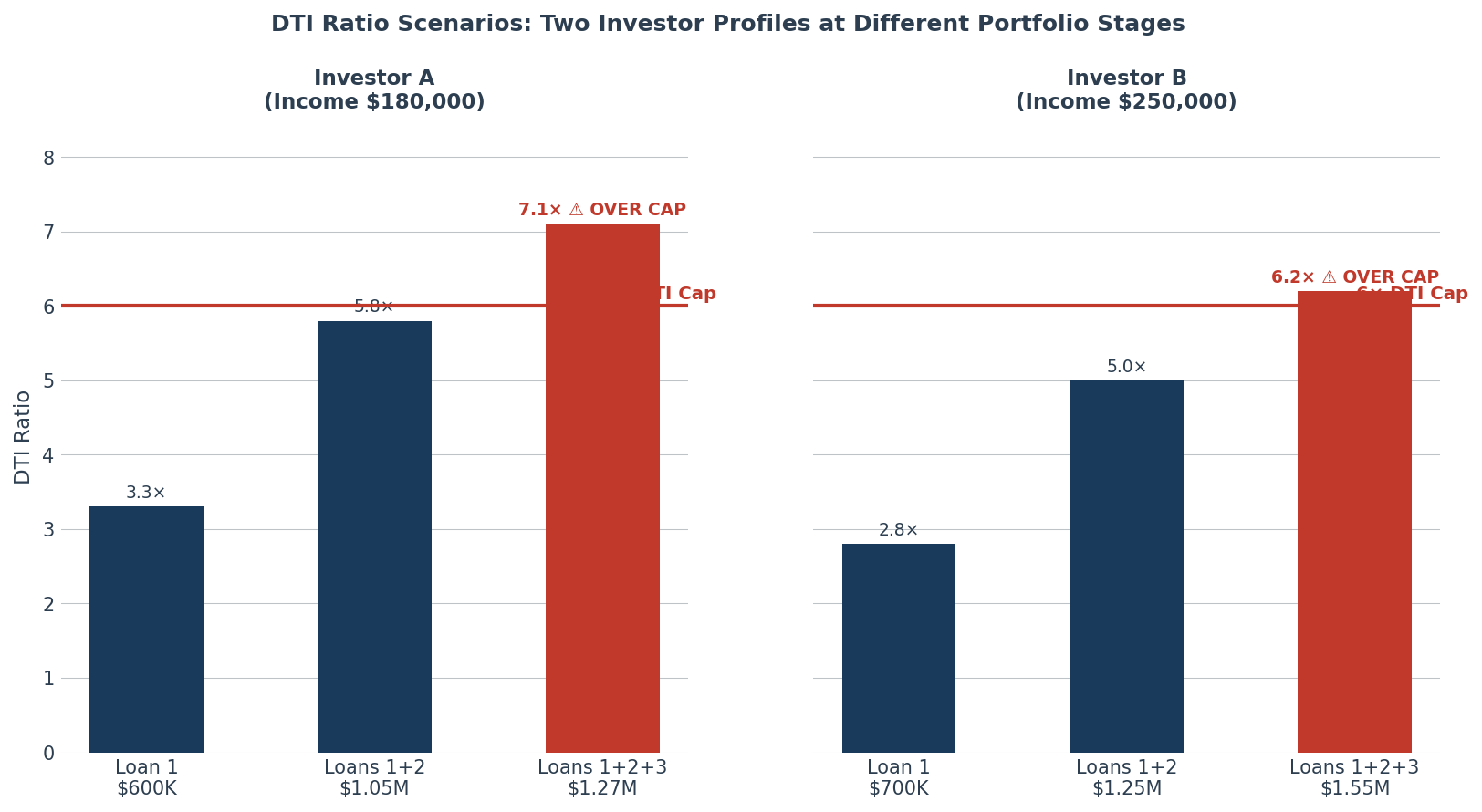
Neither investor approached the six-times DTI threshold at their first acquisition — the constraint appears gradually, one property at a time. Investor A (income $180,000) crosses the cap at their third loan despite a profile that would appear comfortably serviceable on income alone.
The DTI cap does not discriminate by income level. Scale-invariance is a design feature: the same ratio applies equally at $180,000 and $350,000 income.
Source: Modelled scenario. APRA DTI cap framework, February 2026.
What This Means in Practice
Most investors do not know they are approaching the DTI cap until a loan application returns unexpectedly. By then, the options narrow considerably.
The practical solution is to calculate both DTI and serviceability at the time of every acquisition, before committing to a purchase.
For investors already above six times, the path forward runs through income growth, debt reduction, or a shift toward new construction where the cap exemption applies.
How Equity Affects Borrowing Capacity
The relationship between equity and borrowing capacity is widely misunderstood. It tends to surface at the most inconvenient moment, when an investor has accumulated meaningful equity and assumes it translates directly into available credit.
It does not. Equity solves the deposit problem; it does not solve the income problem.
Borrowing capacity is determined by the surplus income remaining after all existing debt obligations are serviced at the stress-test rate. Equity that sits in a property cannot be serviced against. Only income can.
How Equity Access Interacts with Borrowing Constraints
Using equity to buy investment property is how most Australian investors fund their second and third acquisitions. A property purchased for $700,000 five years ago, now valued at $950,000 with $480,000 in outstanding debt, holds approximately $280,000 in useable equity at an 80 per cent LVR ceiling.
But drawing down that equity requires a refinance or supplementary facility that increases total debt. Total debt increasing moves the DTI ratio upward. The additional debt obligation enters the stress-test model, reducing the surplus available to service the next loan.
The equity is real and accessible. Accessing it has a cost in borrowing capacity terms that does not show up in the equity calculation itself. A well-structured equity investment strategy runs the serviceability model on the post-access position before executing the refinance, not after.
Equity growth is not the same as borrowing capacity growth. Investors who conflate the two tend to over-estimate their ability to scale in the near term.
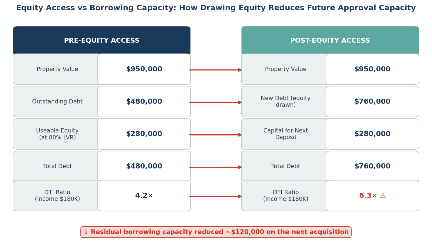
Accessing $280,000 in useable equity provides the deposit for the next acquisition, but it simultaneously increases total debt from $480,000 to $760,000. This pushes the DTI ratio from 4.2 times to 6.3 times on an $180,000 income. That single transaction moves the investor from comfortable headroom below the DTI cap to above it, reducing residual borrowing capacity for the subsequent acquisition by approximately $120,000.
The equity is real. The cost of accessing it in capacity terms does not appear in the equity calculation itself.
Source: Modelled scenario under standard LVR and DTI calculations. APRA DTI framework, February 2026.
What This Means in Practice
The more useful mental model is to track useable equity and residual borrowing capacity separately.
Useable equity is what you have for deposits. Residual borrowing capacity is what the bank will actually approve on your current income.
The gap between the two defines the real constraint. Running both numbers before each decision, not just one, is the starting point. See also: how to build a property portfolio using equity.
Why Property Investors Hit Lending Limits
The pattern repeats across investor cohorts with enough consistency to be analysed structurally. Investors build through the first two acquisitions with relative ease, and then encounter a ceiling that arrives without the warning signs they expected.
The Architecture of the Ceiling
Three percentage points of serviceability buffer assessed across a growing portfolio compounds with every new loan. Rental income accepted at a discount means the portfolio's own cash flows contribute less to the serviceability model than actual performance suggests they should.
Living expense benchmarks rise with income, reducing assessed surplus even as earnings grow. And since February 2026, the DTI framework operates as a second structural ceiling on top of all of that.
Australian household debt now sits at approximately 112 per cent of GDP, among the highest in the developed world. That is the context APRA is managing.
From APRA's perspective, the lending limits it has maintained and extended are a response to a systemic structural condition, not an overreaction to a temporary episode. The settings are not primarily a response to the market cycle. Understanding that framing removes the expectation that regulatory settings will relax as property market conditions improve. See also: property investment risk.
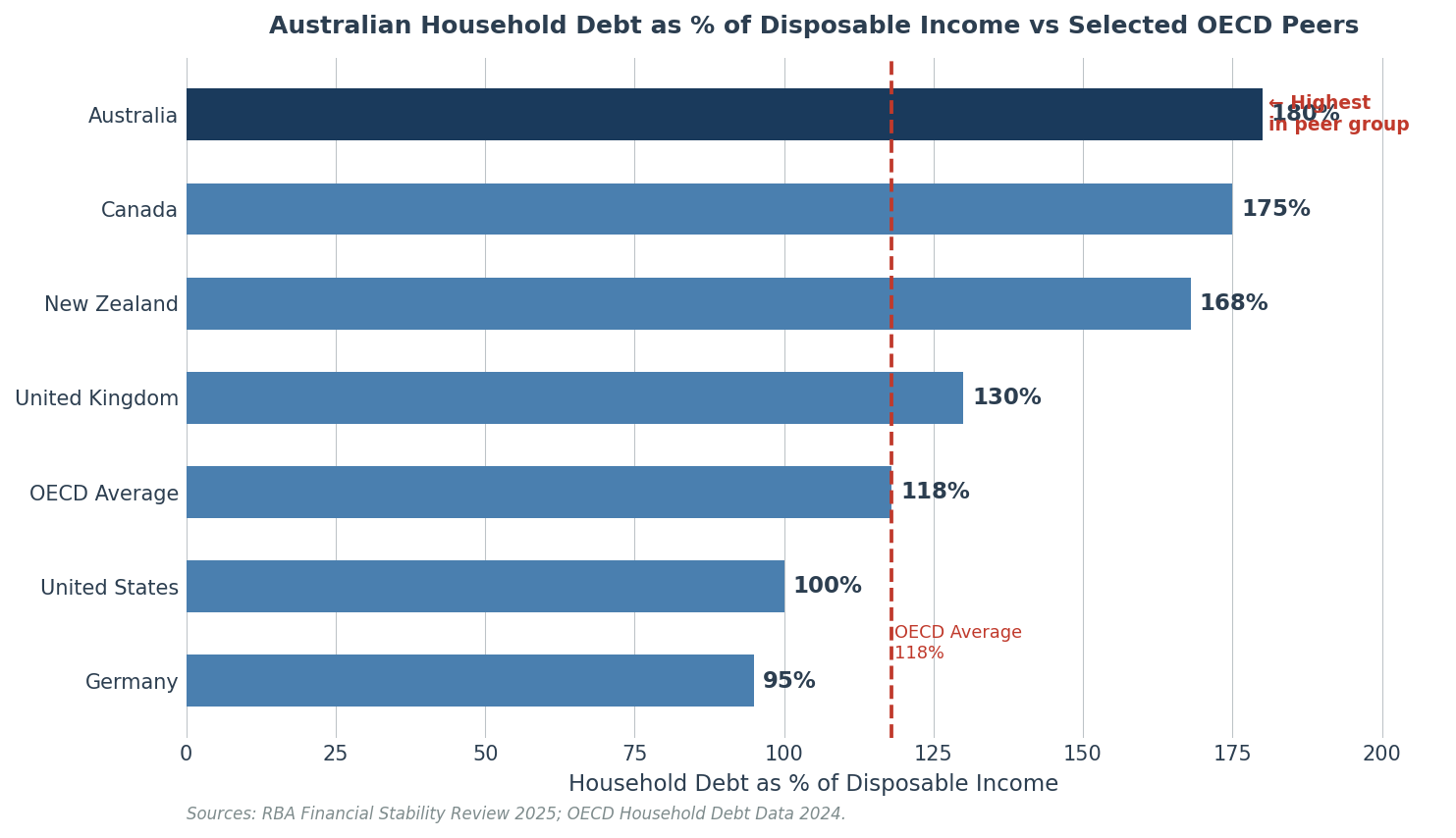
At 180 per cent of disposable income, Australian household debt is the highest in this peer group, above Canada (175 per cent), New Zealand (168 per cent), and more than 60 percentage points above the OECD average.
This is the systemic condition APRA is managing. The lending controls introduced since 2014 are a rational institutional response to a structural imbalance that has persisted for more than two decades.
Investors who expect regulatory settings to soften as property market conditions improve are misreading the policy posture. APRA is responding to the debt stock, not the property cycle.
Source: RBA Financial Stability Review 2025. OECD Household Debt Data 2024.
What Lenders Are Doing Beyond APRA's Formal Requirements
Individual lenders have introduced credit policy changes that go beyond what APRA mandates. Some have restricted investor lending through discretionary trust structures. Others apply lower rental income acceptance rates for investors with more than four properties. Property portfolio stalling at two properties is, in many cases, encountering lender-specific policy rather than a fundamental capacity limit.
None of these changes are published in product guides. They appear as outcomes, applications that would have been approved six months ago returning with different results today.
The solution in those cases is often lender selection rather than balance sheet restructuring. The investment mistakes investors make after the first property frequently concentrate at exactly this junction.
What This Means in Practice
When a loan application returns unexpectedly, the first question should not be whether the portfolio is too large.
It should be whether this is a fundamental serviceability or DTI constraint, or a lender-specific policy decision.
One requires income or debt restructuring. The other may require nothing more than a different lender.
Borrowing Capacity vs Serviceability
These terms are used interchangeably in most property commentary, broker conversations, and lending product material. They describe different things.
Serviceability is the determination that a borrower can meet repayments on a specific proposed loan under the lender's stress assumptions. It is a pass or fail assessment on a single application.
Borrowing capacity is the maximum loan amount for which that assessment produces a pass. The ceiling, not the threshold.
A borrower can be comfortably meeting every existing loan obligation while having very limited residual capacity to take on new debt. The surplus income remaining after all existing commitments are stress-tested at 9.5 per cent may support only a small additional loan amount.
The ceiling is not arbitrary. It is calculated. Once you understand how it is calculated, the levers available to expand or work within it become legible.
Why the Buffer Creates a Permanent Gap Between Rate Movements and Capacity Recovery
When variable rates fell to 2.5 per cent in 2020 and 2021, the assessment rate under the then-current buffer was approximately 5 per cent. When rates rose to a peak of around 4.35 per cent in late 2023, the assessment rate reached approximately 7.35 per cent.
Rates have since partially retreated. Borrowing capacity does not track interest rate movements symmetrically. Rate rises increase the assessment rate by their full amount. Rate cuts reduce it by their full amount.
But because the buffer is fixed at three points, any environment where actual rates are higher than the low-rate period produces a higher assessment rate and lower borrowing capacity. The RBA rate cycle compressed capacity sharply on the way up. Subsequent cuts have partially restored it. A 50-basis point rate reduction translates into only a 50-basis point reduction in the assessment rate. Meaningful, but not a recovery from the hundreds of basis points of compression that accumulated during the tightening cycle.
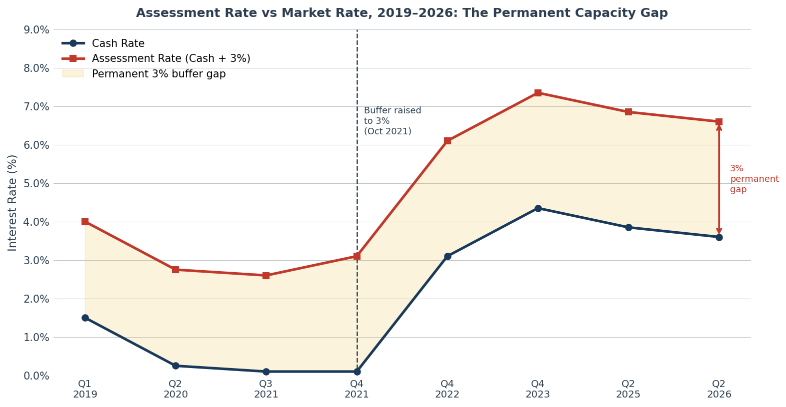
The shaded area between the two lines represents the permanent three-point buffer that separates the rate borrowers pay from the rate they are assessed at, a gap that has never closed and, under current APRA settings, never will.
When the cash rate sat at 0.1 per cent in 2021, the assessment rate was 2.6 per cent. At 3.6 per cent in mid-2026, the assessment rate sits at 6.6 per cent — more than double the pre-2022 assessment level despite rates being well off their 2023 peak. Rate cuts improve borrowing capacity incrementally. They do not restore it to the levels that existed before the buffer increase in October 2021.
Source: RBA cash rate history. APRA serviceability buffer settings 2019 to 2026.
What This Means in Practice
Borrowing capacity and serviceability are different lenses on the same risk. Serviceability is the hurdle. Borrowing capacity is the ceiling above it.
Both can bind, in different ways, on the same application.
Tracking them as separate metrics, and updating both calculations before each acquisition decision, is how investors avoid being surprised late in the process.
Common Borrowing Capacity Mistakes Property Investors Make
Most of the errors here are structural rather than strategic. They are baked into how investors approach finance as a transactional step rather than a continuous portfolio management discipline.
Carrying Credit Card Limits That Serve No Purpose
Credit card limits enter the debt calculation at face value. An investor with $80,000 in credit limits across cards that are rarely used has absorbed $80,000 in assessed debt against facilities generating no return.
Cancelling or consolidating those limits before an application improves both serviceability and DTI simultaneously, at no financial cost.
This is the easiest adjustment available and the most consistently overlooked.
Approaching Each Acquisition Without Modelling the Next One
Every property purchase affects the borrowing capacity calculation for the acquisition that follows it. A high-LVR purchase that maximises exposure in the short term may compress the available credit for the next property by more than the equity gain from appreciation compensates for.
Property investment strategy that sequences acquisitions without modelling their cumulative effect on the bank's credit model tends to produce portfolios that stall below the investor's income capacity.
Mistaking Pre-Approval for Settled Capacity
A home loan pre-approval is an assessment of a specific profile at a specific point in time under a specific set of lender policy conditions. All three of those variables can change between the date of approval and the date of the transaction.
Lender policy shifts in investor credit can occur without public announcement. Pre-approval is a useful indicator of position.
Treating it as a guaranteed outcome and then spending months searching for property is a common source of late-stage transaction failures.
Ignoring the Refinance Window Before Each New Purchase
The three to six months before a new property acquisition are the most productive window for restructuring existing debt. A refinance of investment loans during this window can extend interest-only periods, consolidate facilities, or move to a lender with more favourable investor income treatment.
After the contract is exchanged, the options narrow significantly. The lender assessing the new purchase needs to see the existing debt in its final form.
Restructuring during settlement creates complexity most lenders will not accommodate.
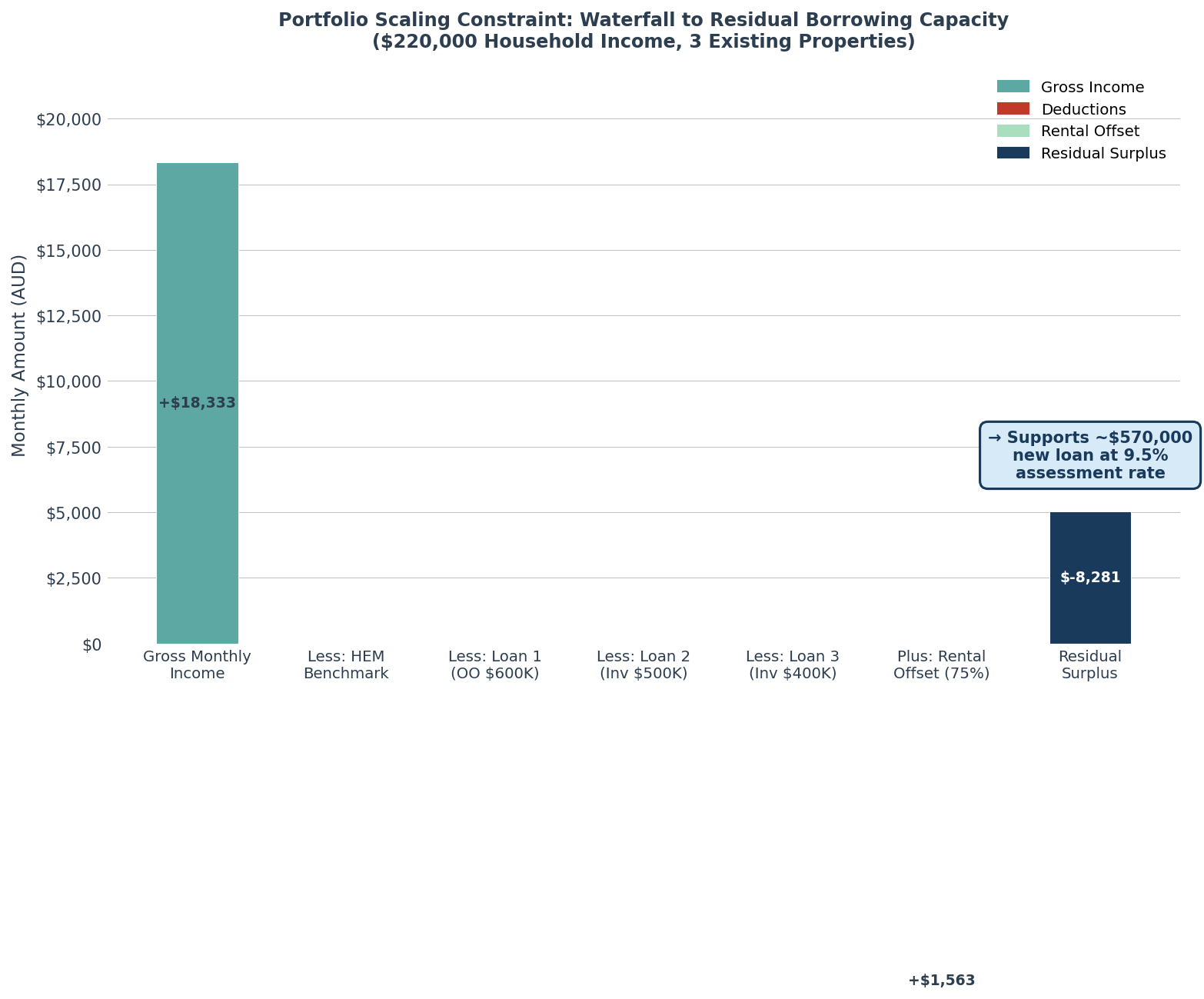
For an investor on $220,000 household income with three existing properties, the bank's model strips away $14,870 per month in stress-tested repayments and living expense benchmarks before assessing what new debt can be added.
The $4,803 monthly surplus that remains supports approximately $570,000 in new lending at the 9.5 per cent assessment rate, a ceiling that bears little relationship to how the portfolio appears on a net worth statement. This is the structural constraint most portfolio investors encounter at the third or fourth acquisition. The ceiling is not arbitrary. It is precisely calculated.
Source: Modelled scenario under standard bank serviceability methodology. APRA HEM benchmark and serviceability buffer settings 2026.
What This Means in Practice
The window for productive finance adjustments closes at contract exchange, not at settlement.
Investors who treat the finance structure as something to fix after a property is secured tend to have fewer options and more expensive ones.
Build the refinance review into the acquisition calendar as a scheduled step before every new purchase, not as an afterthought.
Can You Still Build a Property Portfolio in Australia in 2026?
Yes. The question is whether you are building the right kind of portfolio, in the right sequence, with a finance structure designed for the environment that actually exists.
The lending environment between 2018 and 2021 allowed sequential portfolio building with a degree of ease that the current framework does not replicate. Assessment rates were lower. DTI scrutiny was limited to internal lender preferences rather than system-level caps. Equity growth was compressing LVR ratios faster than serviceability buffers were compressing approved loan sizes.
That combination rewarded relatively unsophisticated approaches to finance. The outcome looked like strategy. Some of it was timing.
That window is gone. The investors starting or growing portfolios now are working with tighter parameters. The parameters require earlier and more deliberate planning to navigate.
Where Viable Paths Exist
Investors operating at DTI levels below four to five times retain genuine headroom under APRA's six-times threshold. Lender competition for strong-income borrowers with well-structured portfolios remains active. The DTI cap constrains the upper end of leverage, not the market as a whole.
The 2026 federal budget's decision to preserve negative gearing on new construction while removing it from established property purchases after July 2027, combined with the DTI cap exemption for new dwelling loans, creates a structural alignment that favours investors oriented toward development and new supply.
For those investors, the regulatory framework is actively accommodating. Buying a second investment property in the current environment requires more deliberate front-end planning. That is the real change.
Strategic portfolio sequencing is achievable. But it requires treating borrowing capacity as a managed resource, one that is planned, tracked, and structured deliberately across the full portfolio, not just at the point of each individual acquisition.
The investors who build sustained portfolios from here will not necessarily be the ones with the highest incomes. They will be the ones who understood their constraints before they needed to.
What This Means in Practice
The finance structure required to build a property portfolio in 2026 is more deliberate than it was in 2020.
That does not make the strategy unworkable. It makes the planning more important.
Investors who model their borrowing capacity across each acquisition, restructure debt in advance, and match lender to income structure will continue to find viable paths forward. Those who do not will encounter the ceiling sooner than expected. See also: overlooked risks when expanding a property portfolio.
Final Thoughts on Borrowing Capacity and Property Investment
Australia's housing affordability problem has two distinct components that are routinely conflated in public commentary. The first is price. The second is finance.
The second problem has worsened independently of the first, driven by regulatory settings that have structurally reduced approved loan amounts even as prices in some markets have softened.
Investors who understand this distinction are better positioned to build around it.
The ceiling is not arbitrary. It is calculable. And once you understand how it is calculated, the levers available to expand or work within it become legible.
The investors navigating this environment effectively share a common characteristic. They are not the ones with the highest incomes or the most equity.
They are the ones treating finance as a discipline, planning lender selection before acquisition, modelling the serviceability implications of each purchase on the next, restructuring existing debt in the window before new applications, and understanding which constraint is actually binding on their specific profile at this specific point in their property portfolio.
The framework is more complex than it was. Complexity rewards understanding.
What This Means in Practice
Borrowing capacity is not a number you receive from a lender. It is a number you can influence.
The earlier you model it across your portfolio, the more options you have.
Structure before purchase. Not after.
Who we work with
Tailored strategy to guiding Australians at every stage of their property journey.
Not Sure Whether DTI or Serviceability Is Limiting You?
Most investors don't discover their borrowing constraint until a lender declines an application or reduces their approved amount.
Before you commit to another property purchase, find out exactly where you stand. Calculate your borrowing capacity now.
If you want to map your borrowing capacity accurately and structure your next acquisition within it, book a strategy call with our team.


© Copyright 2026. FPW. All Rights Reserved.